3 Week4 - Algorithms & Approximations

3.1 Lesson 1 - Algorithms

3.1.1 Shortest Path Problem

Relations <- read.table(
  text = "
From To weight
SL CH 300
SL IN 245
SL LV 263
SL NV 312
CH CL 362
CH IN 201
IN CO 176
IN CI 112
IN LV 114
LV LX 86
LV NV 175
CL CO 142
CL HB 322
CL MT 201
CL CN 251
CO CI 105
CI LX 95
CI CN 204
LX CN 177
LX KV 170
KV GR 299
CN MT 157
CN GR 244
CN RI 318
MT HB 213
MT WA 209
GR RI 205
HB WA 120
WA RI 111
", header =T)

net <- graph_from_data_frame(Relations, directed=F)


#TODO Erro no pacote
# plot(net,vertex.label.cex = 0.8 , vertex.color=Relations$From, edge.label=Relations$weight,
#      edge.label.cex = 0.8, edge.color = "gray70", edge.label.color = "black")
# 
# 
# as_edgelist(net, names=T)
# as_adjacency_matrix(net, attr="weight")
# 
# as_data_frame(net)

#Plot the degree distribution for our network:
deg <- degree(net, mode="all")
deg.dist <- degree_distribution(net, cumulative=T, mode="all")
plot(x=0:max(deg), y=1-deg.dist, pch=19, cex=1.2, col="orange", 
      xlab="Degree", ylab="Cumulative Frequency")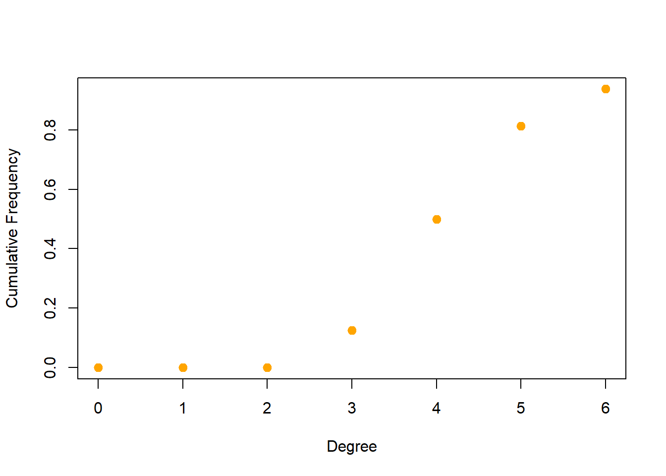

#Shortest Path
sPath <- function(net, from, to){

#Function created based on https://kateto.net/tutorials/  
  
Path <- shortest_paths(net, from = from, to = to, weights = E(net)$weight, output = "both")

# Generate edge color variable to plot the path:

ecol <- rep("gray80", ecount(net))
ecol[unlist(Path$epath)] <- "orange"

# Generate edge width variable to plot the path:

ew <- rep(2, ecount(net))
ew[unlist(Path$epath)] <- 4

 #Generate node color variable to plot the path:

vcol <- rep("gray40", vcount(net))
vcol[unlist(Path$vpath)] <- "gold"

#plot

plot(net, vertex.color=vcol, edge.color=ecol,
     edge.width=ew, edge.arrow.mode=0)

}


sPath(net, from = "LV", to =  "WA")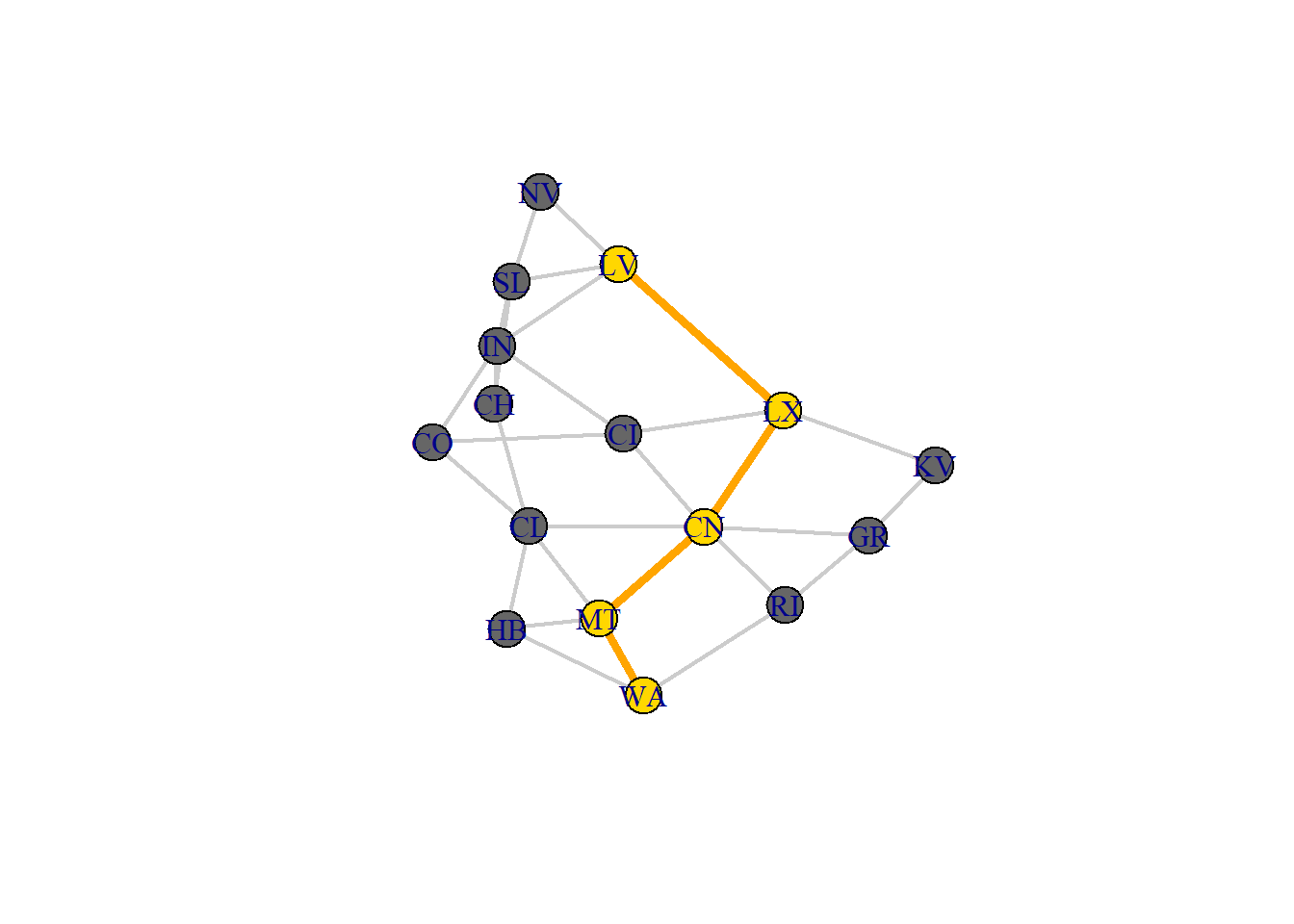

All lowest distances from the model

# all vertices to all vertices

distMatrix <- shortest.paths(net, v=V(net), to=V(net), weight = net$weight)
kable(distMatrix, caption = "Lowest distance from node to node") %>%
  kable_styling() %>%
  scroll_box(width = "100%")

Table 3.1: Lowest distance from node to node

	SL	CH	IN	LV	CL	CO	CI	LX	KV	CN	MT	GR	HB	WA	NV	RI
SL	0	300	245	263	563	421	357	349	519	526	683	770	885	892	312	844
CH	300	0	201	315	362	377	313	401	571	517	563	761	684	772	490	835
IN	245	201	0	114	318	176	112	200	370	316	473	560	640	682	289	634
LV	263	315	114	0	428	286	181	86	256	263	420	507	633	629	175	581
CL	563	362	318	428	0	142	247	342	512	251	201	495	322	410	603	521
CO	421	377	176	286	142	0	105	200	370	309	343	553	464	552	461	627
CI	357	313	112	181	247	105	0	95	265	204	361	448	569	570	356	522
LX	349	401	200	86	342	200	95	0	170	177	334	421	547	543	261	495
KV	519	571	370	256	512	370	265	170	0	347	504	299	717	615	431	504
CN	526	517	316	263	251	309	204	177	347	0	157	244	370	366	438	318
MT	683	563	473	420	201	343	361	334	504	157	0	401	213	209	595	320
GR	770	761	560	507	495	553	448	421	299	244	401	0	436	316	682	205
HB	885	684	640	633	322	464	569	547	717	370	213	436	0	120	808	231
WA	892	772	682	629	410	552	570	543	615	366	209	316	120	0	804	111
NV	312	490	289	175	603	461	356	261	431	438	595	682	808	804	0	756
RI	844	835	634	581	521	627	522	495	504	318	320	205	231	111	756	0

3.1.1.1 Dijkstra’s Algorithm

• Inputs: n Connected graph with nodes and arcs with positive costs, d(ij) n Source (s) and Terminal (t) nodes

• Algorithm:

1. for all nodes in graph, set L()=∞, P()=Null, S()=0

2. set s to i, S(i)=1, and L(i)=0

3. For all nodes, j, directly connected (adjacent) to node i, if L(j) > L(i) + d(ij), then set L(j) = L(i) + d(ij) and P(j)=i

4. For all nodes where S()=0, select the node with lowest L() and set it to i, set S(i)=1

5. Is this node t, the terminal node? If so, go to end If not, go to step 3

6. end – return L(t)

The shortest_path and shortest.path function already solves it by default with dijkstra’s model when the weights have only positive values.

But let’s mimic the algorithm and try to get the results.

Djikstraz <- function(net, source, terminal){

source <- 1
terminal <- 7
  
data <- as.matrix(as_adjacency_matrix(net, attr="weight"))

n = nrow(data)
M = 10000000 

iMin = 1

data <- cbind(data, L = M)
data <- cbind(data, P = 0)
data <- cbind(data, S = 0)

data[source, "S"] = 1
data[source, "L"] = 0

i = source

while (i != terminal) {
    print(i,terminal)
    for (j in 1:n) {
      print(paste0("j = ",j))
        if (data[j, "L"] > 0) {
          if (data[j, "L"] == data[i, "L"] + data[i, j]) {
              data[j, "L"] <- data[i, "L"] + data[i, j]
              data[j, "P"] <- i
          }
        }
    }
  
  Min <- M
  
  for (i in 1:n) {
    if (data[i, "S"] == 0) {
      if (data[i, "L"] < Min) {
        Min <- data[i, "L"]
        iMin <- i
      }
    }
  }
  
  i <- iMin
  data[i, "S"] = 1

}

data
}

3.1.1.2 LP

$$ \[\begin{align*} \textbf{Minimize} & \ z = \sum_{i=1}^{N} \sum_{j=1}^{M} c_{i,j} \cdot x_{i,j} \\ \textbf{subject to} \\ & \sum_{i=1}^{N} \sum_{j=1}^{M} x_{i,j} - x_{j,i} = 0, \ \forall j \neq s, \ j \neq t \\ & \sum_{i=1}^{N} x_{i,j} = 1, \ \forall j = t \\ & \sum_{i=1}^{N} x_{j,i} = 1 \ \forall j = s \\ & x_{i} \ge 0 \\ \textbf{Where} \\ & x_{i,j} = \text{Number of units flowing on nodes} \\ & c_{i,j} = \text{Cost per unit for flow} \\ & s = \text{Source node} \\ & t = \text{Terminal node} \end{align*}\] $$

3.1.2 Traveling Salesman Problem

3.1.2.1 Nearest Neighbor

3.1.2.2 2-opt

3.1.3 Vehicle Routing Problem

3.1.3.1 Sweep Heuristic

3.1.3.2 Clark-Wright

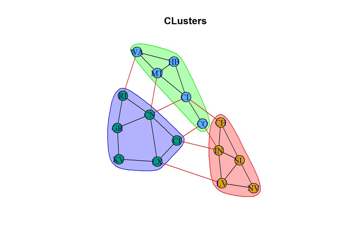
Cool way to create the clusters based on the distance weights, clustering based on the lowest interconnected nodes distance. This is cool because we don’t have to define the number of clusters, it will define it by the distance parameter

# edge betweenness
ceb <- cluster_edge_betweenness(net, weights = Relations$weight)

#Dendogram
dendPlot(ceb, mode="hclust")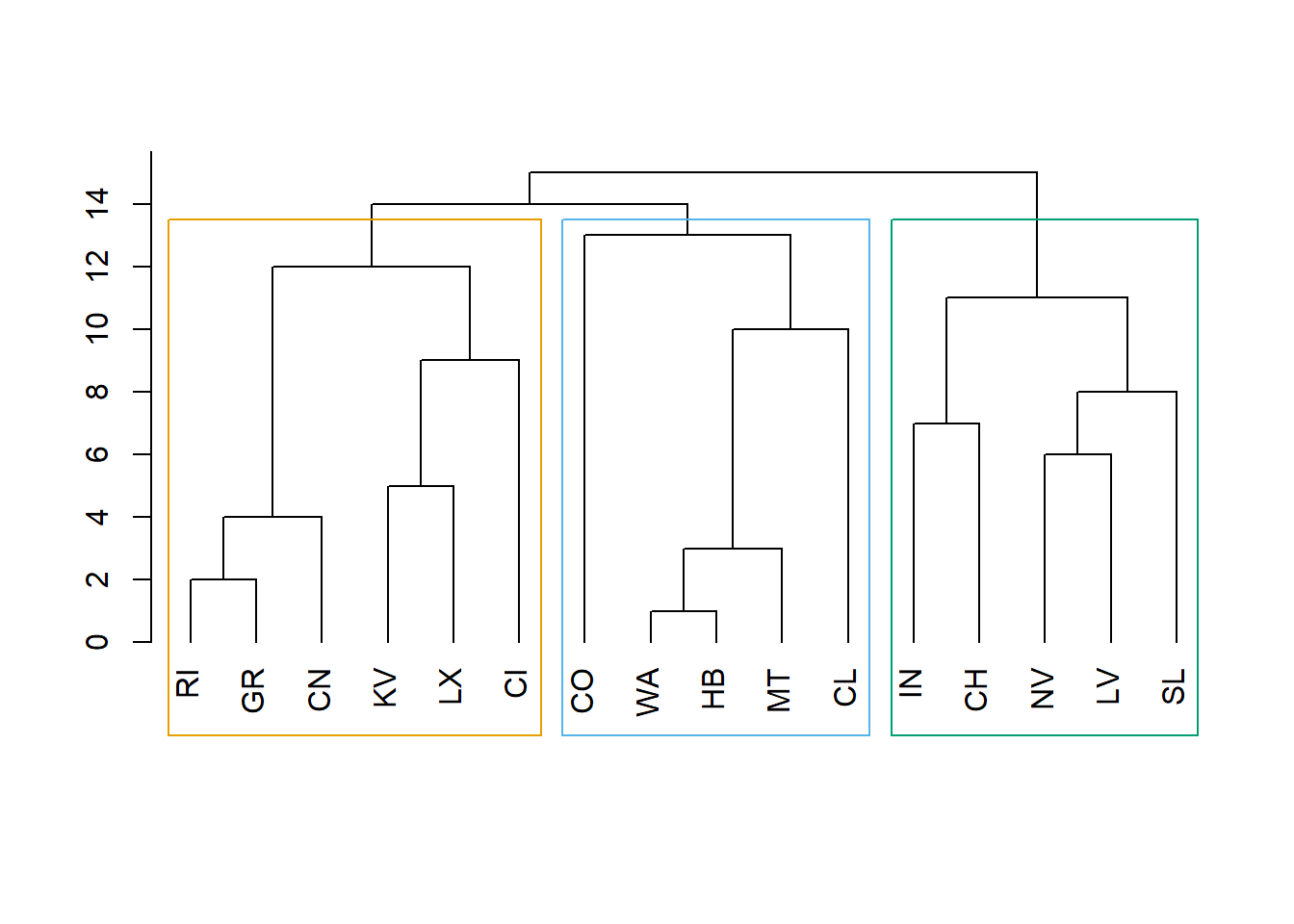

#Graph Plot
plot(ceb, net, main = "CLusters") 

3.1.3.3 MILP